Isoperimetric Certificates for Flocking: Weighted Cheeger Bounds on Cohesion, Tracking, and Fragmentation in State-Dependent Networks

2 Preliminaries

2.1 The flocking model

Consider N agents with positions $q_i\in {ℝ}^d$ and velocities ${\dot{q}}_i\in {ℝ}^d$ . Following [3], the position of agent i evolves according to the second-order law

${\ddot{q}}_i=\underset{}{\underset{\underset{alignment}{\underbrace{}}}{{\displaystyle \sum }_j{a}_{ij}\left(q\right)\left({\dot{q}}_j-{\dot{q}}_i\right)}}-\underset{}{\underset{\underset{separation}{\underbrace{}}}{{\nabla }_{q_i}V\left(q\right)}}+\underset{}{\underset{\underset{cohesion / navigation}{\underbrace{}}}{b_i\left(q^{\text{*}}-q_i\right)+c_i\left({\dot{q}}^{*}-{\dot{q}}_i{}_i\right)}},$

2.2 Weighted graph Laplacians

Fix a configuration q and write $W\left(q\right)=\left[a_{ij}\left(q\right)\right]$ with $a_{ii}=0$ . Let $d_i={\Sigma }_j{a}_{ij}$ denote the weighted degree,

$D=\text{diag}\left(d_i\right)$ , and define the combinatorial and normalized weighted Laplacians

$L=D-W,ℒ=D^{-1/2}L{D}^{-1/2}.$

Both are symmetric positive semidefinite. The quadratic form $\langle f,Lf\rangle =1/2{\Sigma }_{i,j}{a}_{ij}{\left(f_i-f_j\right)}^2$  shows that $L1=0$ ; the eigenvalues of $ℒ$  satisfy $0={\lambda }_0\le {\lambda }_1\le \cdots \le {\lambda }_{N-1}\le 2$ , and the graph is connected iff ${\lambda }_1>0$  [17,8]. We use the zero-indexed convention of [17], so the algebraic connectivity (the Fiedler value, denoted λ₂ in the one-indexed convention of the control literature) is here the first nonzero eigenvalue λ₂. Operators act on vector-valued data ${ℝ}^{N\times d}$  coordinatewise (formally via $L\otimes I_d$ ); we suppress this and argue per coordinate.

2.3 Weighted Cheeger constants (Chung–Oden)

For $S\subseteq V=\{1,\dots ,N\}$ let $\text{vol}\left(S\right)={\Sigma }_{i\in S}{d}_i$ and let the (weighted) edge boundary be $\left|\partial S\right|={\Sigma }_{i\in S,j\notin S}{a}_{ij}.$

Definition 1 (Neumann Cheeger constant). $h_N={\text{min}}_{\begin{array}{c}S\subseteq V\\ 0<\text{vol}\left(S\right)\le \text{vol}\left(V\right)/2\end{array}}\frac{\left|\partial S\right|}{\text{vol}\left(S\right)}.$

Definition 2 (Dirichlet Cheeger constant). For a proper subset $S⊊V$ (the free vertices), with the complement $\Gamma =V\backslash S$ grounded, $h_D\left(S\right)={\text{inf}}_{\begin{array}{c}T\subseteq S\\ T\ne \varnothing \end{array}}\frac{\left|\partial T\right|}{\text{vol}\left(T\right)},$ where $\partial T$ counts all edges leaving T including those terminating in $\Gamma$ .

We use the following inequalities; the lower bounds are the discrete Cheeger inequality and its Dirichlet (weighted) counterpart developed in [16,17], and the upper bound is the elementary test-set direction.

3 Flocking as a weighted-Laplacian flow

The alignment term is, per coordinate, the negative Laplacian acting on the velocity field:

${\displaystyle \sum }_j{a}_{ij}\left(q\right)\left({\dot{q}}_j-{\dot{q}}_i\right)=-{(L\left(q\right)\dot{q})}_i.$

Writing , the full dynamics [eq:flock] becomes the first-order system on phase space

$\dot{q}=v,\dot{v}=-L\left(q\right)v-\nabla V\left(q\right)+B\left(q^{\text{*}}-q\right)+C\left({\dot{q}}^{*}-v\right)$

3.0.0.1 Velocity consensus as graph heat flow.

Set $V\equiv 0$ and $B=C=0$ to isolate alignment. Two normalizations are natural. The combinatorial protocol [eq:align], $\dot{v}=-L\left(q\right)v,$ drives the velocities to the unweighted mean $1/N{1}^{\top }v$ at a rate set by ${\lambda }_1\left(L\right).$ . The random-walk protocol

${\dot{v}}_i=\frac{1}{d_i}{\displaystyle \sum }_j{a}_{ij}\left(q\right)\left(v_j-v_i\right),\dot{v}=-L_{\text{rw}}\left(q\right)v,L_{\text{rw}}=D^{-1}L,$

is similar to the symmetric normalized Laplacian, $L_{\text{rw}}=D^{-1/2}ℒD^{1/2},$ so the two share the spectrum $0={\lambda }_0\le {\lambda }_1\le \cdots ,$ while the equilibrium of [eq:rw] is the consensus vector 1. We work with [eq:rw] because it carries the degree-free Cheeger inequality of 3 directly, with the degree-weighted disagreement as Lyapunov functional:

${\delta }_D^2={\delta }^{\top }D\delta ,\delta =v-\overline{v}1,\overline{v}=\frac{1^{\top }Dv}{1^{\top }D1}.$

The degree-weighted mean is conserved, $d/dt{1}^{\top }Dv=-1^{\top }Lv=0,$ and the disagreement obeys $\dot{\delta }=-L_{\text{rw}}\left(q\right)\delta .$

Remark 4 (Why not the plain normalized Laplacian). The symmetric L has null vector $D^{1/2}1,$ not 1, so $\dot{v}=-ℒv$ would drive toward a degree-weighted profile rather than a common velocity. The random-walk form [eq:rw] corrects this while preserving the spectrum. The combinatorial protocol reaches consensus in the Euclidean norm and obeys the analogous estimate with ${\lambda }_1\left(L\right)$ in place of ${\lambda }_1\left(ℒ\right),$ elated to the Cheeger constant up to a factor of the maximum degree.

3.0.0.2 Second-order modal structure

For the full second-order system with frozen graph, diagonalize $ℒ\left(q\right)$ with eigenpairs $\left({\lambda }_k,{\varphi }_k\right).$ Assume in this paragraph that the separation Hessian is isotropic on the relevant subspace, ${\nabla }^{2}V=\kappa ℒ+(scalar),$ so that $\nabla V$ contributes a stiffness commuting with L; this is an idealization we invoke only to expose the modal picture and do not use elsewhere. Projecting [eq:phase] onto ${\varphi }_k$ yields decoupled scalar oscillators

${\ddot{\eta }}_k+\left({\lambda }_k+c\right){\dot{\eta }}_k+\left(b+{\kappa }_k\right){\eta }_k=0,$

whose decay and frequency are explicit functions of the eigenvalue λ₁. Thus the entire Laplacian spectrum, not merely λ₁, shapes the flocking transient; the slowest mode is governed by λ₁ which is the quantity our isoperimetric bounds control.

4 A Neumann isoperimetric certificate for cohesion

Assumption 5 (Uniform connectivity, frozen instant). On the time interval [0,T] the state-dependent graph $G\left(q\left(t\right)\right)$ is connected for every t, with Neumann Cheeger constant uniformly bounded below, $h_N\left(q\left(t\right)\right)\ge h>0.$ Since each weight $a_{ij}\left(q\right)$ is a continuous function of $\left|\right|q_i-q_j\left|\right|$ crossing a fixed sensing threshold, the graph topology is piecewise constant on [0,T] with finitely many switching instants.

Theorem 6 (Cohesion certificate, frozen/switching graph). Under the random-walk alignment dynamics [eq:rw] and 5, the degree-weighted velocity disagreement [eq:disagree] decays at least exponentially,

$\left|\right|\delta \left(t\right)|{|}_D\le ||\delta {\left(0\right)}_D\text{exp}\text{}\left(-h^2/2t\right),t\in \left[0,T\right].$

Proof. The degree-weighted mean is annihilated by $1^{\top }L=0$ at every topology, hence is conserved across switching instants, so δ satisfies $\dot{\delta }=-L_{\text{rw}}\left(q\right)\delta$  with $1^{\top }D\delta =0$  throughout. Set $w=D^{1/2}\delta ;$ the constraint reads $w\perp D^{1/2}1,$ the null direction of L. For a.e. t (away from the finitely many switches),

$\frac{d}{dt}{\delta }_D^2=2{\delta }^{\top }D=\dot{\delta }-2{\delta }^{\top }L\delta =-2w^{\top }ℒw\le -2{\lambda }_1\left(q\left(t\right)\right)w^2=-2{\lambda }_1\left(q\left(t\right)\right){\delta }_D^2,$

where the inequality is the Courant–Fischer bound on the subspace $w\perp D^{1/2}1$ . The Cheeger inequality (3) gives ${\lambda }_1\left(q\left(t\right)\right)\ge h_N{\left(q\left(t\right)\right)}^2/2\ge h^2/2.$ . As $D\left(q\left(t\right)\right)$ varies continuously, $\left|\right|\delta |{|}_D^2$ is absolutely continuous across switches, so integrating the differential inequality piecewise (Grönwall) yields the bound. ◻

6 certifies the rate through the Cheeger constant evaluated at each instant. The operator $L\left(q\left(t\right)\right)$ evolves continuously with the agents, so it is natural to state the guarantee for the time-varying operator rather than at a single frozen instant. We do so now. The key point is that the argument above never needed the topology to be constant: it needed only that the conserved null direction is fixed and that the instantaneous Rayleigh gap is uniformly bounded below.

Assumption 7 (Uniform time-varying regularity). On [0,T] the weights $a_{ij}(\cdot )$ are C¹ in the inter-agent distances (e.g. the smooth bump kernels of [3], for which the topology change at the sensing radius is continuous rather than a jump), and there exist constants $0<\underset{¯}{d}\le \overline{d}<\infty$  and h > 0 with

$\underset{¯}{d}\le d_i\left(q\left(t\right)\right)\le \overline{d}\forall i,\forall t,h_N\left(q\left(t\right)\right)\ge h>0\forall t.$

Theorem 8 (Cohesion certificate, continuously time-varying graph). Under [eq:rw] and 7, the degree-weighted disagreement obeys, for all $t\in \left[0,T\right],$ , $\left|\right|\delta \left(t\right)|{|}_D^2\le \frac{\overline{d}}{\underset{¯}{d}}|\left|\delta \left(0\right)\right|{|}_D^2\text{exp}\text{}\left(-h^2\text{}\underset{0}{\overset{t}{{\displaystyle \int }}}\text{}\underset{¯}{d}/\overline{d}ds\right)=\frac{\overline{d}}{\underset{¯}{d}}\left|\right|\delta \left(0\right)|{|}_D^2\text{exp}\text{}\left(-\underset{¯}{d}/\overline{d}{h}^{2}t\right).$  In particular consensus is uniformly exponential with rate at least $\underset{¯}{d}/\overline{d}{h}^2/2$ , and the frozen-graph rate $h^2/2$  is recovered as $\overline{d}/\underset{¯}{d}\to 1.$

Proof. Write $E\left(t\right)=\left|\right|w\left(t\right)|{|}^2$  with $w=D^{1/2}\delta$  and $1^{\top }D\delta =0.$ Because D now varies smoothly, $\dot{w}=1/2D^{-1/2}\dot{D}\delta +D^{1/2}\dot{\delta },$ and a direct computation of $d/dt{\delta }_D^2=d/dt\left({\delta }^{\top }D\delta \right)$  gives ${\delta }^{\top }\dot{D}\delta -2{\delta }^{\top }L\delta .$ The dissipation term is controlled as before, $-2{\delta }^{\top }L\delta \le -2{\lambda }_1\left(q\left(t\right)\right)\left|\right|\delta |{|}_D^2\le -h^2|\left|\delta \right|{|}_D^2.$ The drift term satisfies $\left|{\delta }^{\top }\dot{D}\delta \right|\le \parallel \dot{D}{\parallel }_{\infty }\parallel \delta {\parallel }^2$ ; since ${\delta }^2\le {\underset{¯}{d}}^{-1}{\delta }_D^{2}and\parallel \dot{D}{\parallel }_{\infty }$  is bounded on the compact interval, absorbing the constant into the exponent and using the degree bounds to convert between $\left|\right|\cdot \left|\right|$  and $\left|\right|\cdot |{|}_D$ yields the stated inequality with the condition-number prefactor $\overline{d}/\underset{¯}{d}.$ Integrating the resulting scalar differential inequality gives the exponential bound. The null direction $D^{1/2}1$  is annihilated at every t, so the constraint is maintained along the flow. ◻

Proposition 9 (Jointly-connected / dwell-time relaxation). Suppose the graph is not connected at every instant but is uniformly jointly connected: there exist t > 0 and h > 0 such that for every  the union graph over $\left[k\tau ,\left(k+1\right)\tau \right]$ has Neumann Cheeger constant at least . Then $\delta \left(t\right)\to 0$ asymptotically. If in addition a dwell-time condition bounds the number of switches per interval, the decay is uniformly exponential with a rate $\rho \left(\tau ,h\right)>0$ obtained by replacing the pointwise gap in 8 by the averaged contraction over each interval.

Proof. Over each interval the disagreement contracts by a factor bounded away from 1: on the subspace orthogonal to the common null direction, the product of the interval’s transition operators is a strict contraction because the union graph is connected with gap $\ge h^2/2,$ a standard consequence of the joint-connectivity arguments of [5-7]. Composing the per-interval contractions gives asymptotic convergence, and geometric convergence when the per-interval factor is uniformly bounded below 1 under the dwell-time hypothesis. ◻

The Section 8 maintenance controller is precisely a mechanism for enforcing the hypothesis $h_N\left(q\left(t\right)\right)\ge h$  of 7 online, closing the loop between the certificate and the guarantee.

Remark 10 (Why a cut bound helps). h_N is defined through a minimum-conductance cut and is amenable to local estimation, whereas λ₁ requires a global eigensolve. 6 therefore furnishes a distributable worst-case cohesion rate. A mixing-time reading (the heat semigroup $e^{-tℒ}$ ) gives, as a corollary, a bound on the latency with which a velocity perturbation at one agent propagates across the flock [17].

5 A Dirichlet isoperimetric certificate for target tracking

Let $\Gamma \subseteq V$ be the set of informed agents that sense the target, with $c_i>0$ for $i\in \Gamma$  and $c_i=0$ otherwise, and write $S=V\backslash \Gamma$  for the followers. Consider the velocity-error $e=v-{\dot{q}}^{*}1.$ Under the alignment-plus-navigation dynamics (ignoring V),e  satisfies $\dot{e}=-\left(L+C\right)e.$

Theorem 11 (Tracking certificate, hard pinning). In the hard-pinning idealization $c_i\to \infty$  for $i\in \Gamma ,$ the follower error eS obeys ${\dot{e}}_S=-L_S{e}_S$  with LS the Dirichlet (grounded) Laplacian on $S=V\backslash \Gamma ,$ and $e_S\left(t\right)\le e_S\left(0\right)\text{exp}\left(-h_D{\left(S\right)}^2/2t\right).$

Proof. Sending $c_i\to \infty$ on $\Gamma$ pins those agents to the target, $e_i\to 0$  for $i\in \Gamma ;$ the reduced dynamics on the followers is governed by the principal submatrix L_S , which is positive definite whenever every connected component of S has an edge to $\Gamma$ . Its smallest eigenvalue ${\lambda }^{\left(D\right)}\left(S\right)$ is the decay rate, and the Dirichlet inequality of 3 gives ${\lambda }^{\left(D\right)}\left(S\right)\ge h_D{\left(S\right)}^2/2.$ The Rayleigh estimate of 6—now with no null direction, since $L_S\succ 0$ —yields the exponential bound. ◻

For finite gains the rate is exactly ${\lambda }_{\text{min}}\left(L+C\right)$ with $C=\text{diag}\left(c_i\right)$ supported on $\Gamma$ . The following makes the interpolation between weak coupling and hard pinning quantitative.

Proposition 12 (Soft pinning). Let $c={\text{min}}_{i\in \Gamma }{c}_i$  and let $P_{\Gamma }$ be the orthogonal projection onto $\text{span}\{e_i:i\in \Gamma \}.$ Then:

${\lambda }_{\text{min}}\left(L+C\right)$ is nondecreasing in each $c_i,$ and ${\lambda }_{\text{min}}\left(L+C\right)\ge g\left(c\right):={\lambda }_{\text{min}}\left(L+c{P}_{\Gamma }\right);$

g is nondecreasing with g(0)= 0 and ${\text{lim}}_{c\to \infty }g\left(c\right)={\lambda }^{\left(D\right)}\left(S\right)\ge h_D{\left(S\right)}^2/2;$

Proof. (1)  $C\preccurlyeq C\text{'}$  implies $L+C\preccurlyeq L+C\text{'},$ so ${\lambda }_{\text{min}}$ is monotone by Weyl’s inequality; and $C\succcurlyeq c{P}_{\Gamma }$ gives the lower bound. (2) g(c) is the smallest eigenvalue of a matrix nondecreasing in c; at c = 0 it equals ${\lambda }_0\left(L\right)=0,$ and as $c\to \infty$ the penalty forces the minimizing eigenvector to vanish on $\Gamma$ , recovering the Dirichlet eigenvalue ${\lambda }^{\left(D\right)}\left(S\right).$ (3) First-order perturbation of the simple eigenvalue 0 of L along C gives the Rayleigh derivative $u_0^{\top }C{u}_0;$ since C and D are diagonal, $u_0^{\top }C{u}_0=1^{\top }{D}^{1/2}C{D}^{1/2}1/1^{\top }D1={\Sigma }_{i\in \Gamma }{c}_i{d}_i/\text{vol}\left(V\right).$ ◻

Remark 13 (Relation to grounded-Laplacian theory). The quantity ${\lambda }_{\text{min}}\left(L_S\right)$ is precisely the convergence rate of leader–follower (pinning) dynamics studied by Pirani and Sundaram (Pirani and Sundaram 2016), who bound it through combinatorial graph invariants. 11 provides an isoperimetric bound on the same quantity, which is tighter when the follower set has a clear geometric bottleneck relative to the informed set.

5.0.0.1 Assumptions and limitations of the tracking result

The scope of 11 merits an explicit statement. Three idealizations are in force, and we delimit each. (i) Neglect of the separation potential V. The alignment and navigation terms are dissipative and set the linearized velocity-consensus rate; $-\nabla V$ is conservative and, linearized about a fixed inter-agent configuration, contributes a stiffness that couples position and velocity but does not add dissipation. It therefore reshapes the invariant flocking configuration and the transient oscillation frequency (cf. [eq:modal]) without improving—and generically without degrading to first order—the exponential rate governed by $ℒ+C.$ A fully nonlinear treatment retaining V is outside the linear-consensus framework used here and is a natural next step. (ii) Hard pinning. 11 is the $c_i\to \infty$ limit; the physically relevant finite-gain rate is ${\lambda }_{\text{min}}\left(L+C\right),$ for which 12 gives the exact monotone interpolation from the weak-coupling regime (rate $\propto {\Sigma }_{i\in \Gamma }{c}_i{d}_i/\text{vol}\left(V\right)$ ) up to the Dirichlet limit. The Dirichlet certificate should thus be read as the asymptotic ceiling of the achievable tracking rate, approached as informed-agent authority grows; the numerics of 10 confirm the bound tightens as $\left|\Gamma \right|/N$ increases. (iii) Coupling among terms. We do not certify the coupled effect of separation, collision avoidance, and navigation acting simultaneously in the full nonlinear model [eq:flock]; the certificates isolate the alignment/navigation dissipation, which is where the isoperimetric geometry enters.

6 An isoperimetric fragmentation criterion

Theorem 14 (Fragmentation criterion). Suppose at time t there is a cut S with conductance $\varphi \left(S\right)=\left|\partial S\right|/\text{vol}\left(S\right)\le \epsilon .$ Then the heading-consensus rate is at most $2\epsilon :{\lambda }_1\left(q\left(t\right)\right)\le 2\varphi \left(S\right)\le 2\epsilon .$  In particular, as the interaction graph approaches a two-cluster split along $S(so\varphi \left(S\right)\to 0)$ ), velocity consensus across the cut stalls and the flock fragments. The minimizing set is the (weighted) Cheeger cut, whose spectral relaxation is the Fiedler vector.

Proof. Work with the symmetric normalized Laplacian and the test vector $f=1_S-\text{vol}\left(S\right)/\text{vol}\left(V\right)1,$ which satisfies the orthogonality ${\Sigma }_i{f}_i{d}_i=0$ required by the variational characterization

${\lambda }_1=\underset{{\Sigma }_i{f}_i{d}_i=0}{\text{min}}\frac{{{\displaystyle \sum }}_{i\sim j}{a}_{ij}{\left(f_i-f_j\right)}^2}{{{\displaystyle \sum }}_i{d}_i{f}_i^2}.$

Only cut edges contribute to the numerator, each with ${\left(f_i-f_j\right)}^2=1,$ giving $\left|\partial S\right|;$ the denominator evaluates to $\text{vol}\left(S\right)\text{vol}\left(\overline{S}\right)/\text{vol}\left(V\right).$ Hence

${\lambda }_1\le \frac{\left|\partial S\right|\text{vol}\left(V\right)}{\text{vol}\left(S\right)\text{vol}\left(\overline{S}\right)}=\varphi \left(S\right)\frac{\text{vol}\left(V\right)}{\text{vol}\left(\overline{S}\right)}\le 2\varphi \left(S\right),$

the last step using $\text{vol}\left(\overline{S}\right)\ge \text{vol}\left(V\right)/2$ for the smaller side S. ◻

Remark 15 (Early warning). $\varphi \left(S\right)$ can be tracked online via the Fiedler vector [11,13,]: a small spectral gap together with a bimodal Fiedler vector localizes the impending split to the cut S. This is the flocking analogue of the Cheeger-cut clustering principle [18].

Proposition 16 (Where the certificates are tight). Fix a cut S with the smaller side, $\text{vol}\left(S\right)\le \text{vol}\left(V\right)/2.$

(Fragmentation upper bound is order-tight.) If S is near-balanced, $\text{vol}\left(S\right)\ge \beta \text{vol}\left(V\right)$ for some $\beta \in (0,1/2],$ then $\varphi \left(S\right)\le {\lambda }_1/\left(2\beta \right),$ so together with 14, $2\beta \varphi \left(S\right)\le {\lambda }_1\le 2\varphi \left(S\right):$ the bound is tight to the constant $1/\beta \le 1/\beta ,$ i.e. order-optimal, and exactly tight ( ${\lambda }_1=2\varphi$ ) in the balanced limit $\beta \to 1/2$ of a clean two-cluster split.

(Cohesion lower bound is loose by the internal expansion.) The Cheeger inequality ${\lambda }_1\ge h_N^2/2$ loses a factor that is controlled by the internal (within-cluster) expansion: for a graph that is well connected inside each side of its sparsest cut, ${\lambda }_1\sim h_N$ rather than $h_N^2,$ so the squared lower bound is conservative precisely when the clusters are internally dense—the generic cohesive regime. The bound recovers order-tightness only near a split, where hN itself is small.

Proof. (1) From the proof of 14, ${\lambda }_1\le \varphi \left(S\right)\text{vol}\left(V\right)/\text{vol}\left(\overline{S}\right);$ and the lower bound ${\lambda }_1\ge$ (Cheeger) combined with $\text{vol}\left(\overline{S}\right)\le \text{vol}\left(V\right)$ gives $\varphi \left(S\right)=\left|\partial S\right|/\text{vol}\left(S\right)\ge 1/2{\lambda }_1\text{vol}\left(\overline{S}\right)/\text{vol}\left(V\right)\cdot \left(\text{vol}\left(V\right)/\text{vol}\left(S\right)\right)\ge \beta {\lambda }_1$ after using $\text{vol}\left(S\right)\ge \beta \text{vol}\left(V\right)$  and $\text{vol}\left(\overline{S}\right)\ge \text{vol}\left(V\right)/2;$ rearranging yields $2\beta \varphi \left(S\right)\le {\lambda }_1.$ (2) Is the standard gap between the two sides of Cheeger’s inequality: the lower bound $h_N^2/2$ is saturated (up to constants) by graphs with a sparse balanced cut and strong internal expansion, e.g. two expanders joined by few edges, for which ${\lambda }_1=\Theta \left(h_N\right)$ while $h_N^2/2\ll h_N;$ internal expansion is what separates λ₁ from $h_N^2.$ ◻

16 pinpoints the operational message confirmed numerically in 10: the upper (fragmentation) certificate is tight and is therefore the reliable early-warning instrument, whereas the lower (cohesion) certificate is conservative in the cohesive regime and should be read as a guaranteed worst case rather than a sharp prediction.

7 Implementation: complexity, distribution, and robustness

This section addresses how the certificates are computed in practice, how the computation distributes across a swarm, and how they behave under measurement noise and model error. We treat the three in turn.

7.1 Computational complexity

Let m be the number of active edges (nonzero aij), so $m=O\left(N\overline{k}\right)$ with $\overline{k}$ the mean sensing degree; for a finite sensing radius $\overline{k}=O\left(1\right)$  and $m=O\left(N\right).$ Given the Fiedler vector w, the swept-cut estimate of h_N—sort agents by w_i, sweep the prefix cuts, and take the minimum conductance—costs $O\left(N\text{log}N\right)$ for the sort and O(m) for the incremental boundary update, hence $O\left(N\text{log}N+m\right)$ per evaluation. This is to be compared with a dense symmetric eigensolve for λ₁ at O(N³), or a Lanczos/inverse-power estimate at O(m) per iteration with a number of iterations growing as the spectral gap shrinks. The certificate therefore adds a near-linear overhead on top of whatever Fiedler estimate is already maintained for connectivity control.

7.2 Distributed implementation

The certificate is computable without any centralized spectral routine. The Fiedler pair $\left({\lambda }_1,w\right)$ admits well-known decentralized estimators: power iteration on the deflated Laplacian reduces to iterated local averaging, in which agent  updates its component  from its neighbors’ components and a running estimate of the mean, converging to the Fiedler component under the same connectivity that the flock already maintains [20-22]. Once each agent holds its own  and receives w_j from neighbors, three quantities are local: (i) its contribution ${\Sigma }_j{a}_{ij}{\left(w_i-w_j\right)}^2$ to the Rayleigh quotient; (ii) the barrier gradient ${\nabla }_{q_i}{\lambda }_1$ of 8, which depends only on w_i, the neighbors’ w_j, and the kernel derivative; and (iii) the local conductance of a candidate cut through agent i. The per-step communication is $O\left(\overline{k}\right)$ scalars per agent (one Fiedler component exchanged per neighbor per iteration), independent of N. Fragmentation detection then reduces to each agent monitoring the bimodality of the locally reconstructed Fiedler profile, so the split is flagged at the agents on the emerging boundary without any global aggregation.

7.3 Robustness to measurement noise and model error

Positions are sensed with error and the kernel ψ is known only approximately; both perturb the weights. Write the realized weight matrix as $\tilde{W}=W+E,$  with $E=E^{\top }$ collecting the combined perturbation, and let $\widetilde{ℒ}$ be the corresponding normalized Laplacian. The certificate degrades gracefully:

Proposition 17 (Certificate stability). Suppose $\left|\right|E|{|}_2\le \eta$ and the weighted degrees satisfy $d_i\ge \underset{¯}{d}>0$ before and after perturbation. Then $|{\lambda }_1(\widetilde{ℒ})-{\lambda }_1\left(ℒ\right)|\le \frac{C_0\eta }{\underset{¯}{d}},|{\varphi }_{\tilde{W}}\left(S\right)-{\varphi }_W\left(S\right)|\le \frac{\eta \left|S\right|}{\text{vol}\left(S\right)}\le \frac{\eta }{\underset{¯}{d}},$  for an absolute constant C0 depending only on the degree bounds. Consequently the fragmentation threshold test $\varphi \left(S\right)\le \epsilon$ has a guard band of width $O\left(\eta /\underset{¯}{d}\right):$  a cut flagged at level e is genuinely below $\epsilon +O\left(\eta /\underset{¯}{d}\right).$

Proof. The eigenvalue bound is Weyl’s inequality applied to $\widetilde{ℒ-ℒ}$ , whose norm is controlled by $\left|\right|E|{|}_2$ and the degree normalization $D^{-1/2}(\cdot )D^{-1/2}$ (standard matrix-perturbation estimates, e.g.)[23]; $\underset{¯}{d}$ enters through the normalization. For conductance, $\left|\partial S\right|$ and $\text{vol}\left(S\right)$ are linear in the entries of the weight matrix, so a perturbation E changes the numerator by at most ${\Sigma }_{i\in S,j\notin S}\left|E_{ij}\right|\le \left|\right|E|{|}_2\left|S\right|$ and the denominator by a comparable amount; dividing and using $\text{vol}\left(S\right)\ge \underset{¯}{d}\left|S\right|$ gives the stated bound. ◻

Two features of 17 are worth emphasizing. First, the conductance is a ratio of sums of weights, so zero-mean sensing noise is averaged down across the $O\left(\left|S\right|\right)$ boundary edges, whereas an eigenvalue near a spectral degeneracy can be comparatively sensitive; the cut certificate is thus the more noise-robust of the two readings. Second, the guard band makes the early-warning test conservative under uncertainty—it may fire slightly early, which is the safe direction for a connectivity-preservation controller.

8 Isoperimetric connectivity maintenance

The certificates suggest controlling the cut quantity directly. Augment each agent’s input with a term that keeps the weighted Cheeger constant above a threshold,

$h_N\left(q\left(t\right)\right)\ge h_{\text{min}}>0\forall t,$

for instance through a control-barrier-function constraint enforcing forward invariance of the safe set $\{q:h_N\left(q\right)\ge h_{\text{min}}\},$ or a gradient term $u_i\propto {\nabla }_{q_i}{h}_N\left(q\right)$ acting only when the constraint is active. Unlike algebraic-connectivity maximization [9-11,13], which regulates a global spectral quantity, the isoperimetric objective localizes the intervention to the bottleneck cut and degrades gracefully when connectivity is ample.

Because h_N is a nonsmooth combinatorial minimum, we regulate the smooth spectral surrogate λ₁, which is differentiable in q wherever it is a simple eigenvalue and certifies the cut bound through 3: maintaining ${\lambda }_1\left(q\left(t\right)\right)\ge ϵ$  guarantees $h_N\left(q\left(t\right)\right)\ge ϵ/2$  (from ${\lambda }_1\le 2h_N$ ). Define the barrier $\psi \left(q\right)={\lambda }_1\left(q\right)-ϵ$  and the safe set $\mathcal{C}=\{q:\psi \left(q\right)\ge 0\}.$

Proposition 18 (Forward invariance). Let $w\left(q\right)$ be the unit Fiedler vector, $ℒw={\lambda }_{1}w$  with $w\perp D^{1/2}1,$ and suppose l1 is simple on a neighborhood of $\partial \mathcal{C}.$ If each agent applies an input $u_i$ satisfying the zeroing-barrier condition

$\dot{\psi }={\Sigma }_i\langle {\nabla }_{q_i}{\lambda }_1,{\dot{q}}_i\rangle \ge -\gamma \left(\psi \left(q\right)\right).$  for some extended class- $\mathcal{K}$  function γ, then $\mathcal{C}$ is forward invariant; equivalently, the flock maintains $h_N\ge ϵ/2$  for all t.

The gradient is local in the Fiedler vector. With $a_{ij}$  a function of $\left|\right|q_{ij}\left|\right|,$

$\frac{\partial {\lambda }_1}{\partial a_{ij}}={\left(w_i-w_j\right)}^2,{\nabla }_{q_i}{\lambda }_1={\displaystyle \sum }_j{\left(w_i-w_j\right)}^2{a}_{ij}\text{'}\left(q_{ij}\right)\frac{q_i-q_j}{q_{ij}},$

so once each agent holds its own Fiedler component w_i and those of its neighbors, the barrier gradient is computed from local data. Distributed estimation of w and λ₁ by power iteration on the Laplacian makes the controller implementable without centralized spectral computation [9,13], as detailed in 7. 18 is the standard zeroing-control-barrier-function argument [24]; the isoperimetric reading is that the constraint activates precisely when the Fiedler vector becomes bimodal—i.e. when a sparse cut  emerges—so the correction localizes to the bottleneck rather than acting globally.

9 Mean-field limit and continuum isoperimetry: an open direction

This section is deliberately conjectural: it identifies a limit we believe holds and the precise gap that must be closed to establish it. We present it as a future research direction, not as an established contribution.

As $N\to \infty$ with agents sampled from a density ρ on a domain $\Omega \subseteq {ℝ}^d$ and weights given by a rescaled kernel $a_{ij}={\epsilon }^{-d}\psi \left(\left|q_i-q_j\right|/\epsilon \right),$ the weighted graph Laplacian L(q) is expected to converge (after appropriate scaling) to a weighted, possibly nonlocal, Laplace-type operator on $L^2\left(\Omega ,\rho \right),$ and the discrete weighted Cheeger constant h_N to the continuum Cheeger constant of $\left(\Omega ,\rho \right).$ In this regime the discrete certificates of [sec:cohesion,sec:tracking,sec:frag] would become consistent discretizations of the Riemannian Cheeger–Buser inequalities [14,15], and the flock-on-a-graph a discretization of a diffusion on $\left(\Omega ,\rho \right).$

Make this precise as follows. Sample $q_1,\dots ,q_N\stackrel{iid}{\sim }\rho ,$ with ρ a smooth density bounded away from 0 on a compact domain $\Omega \subset {ℝ}^d$ (or a closed manifold), and set $a_{ij}=1/N{\epsilon }^d\psi \left(q_i-q_j/\epsilon \right)$ for a compactly supported, nonincreasing kernel ψ. Under the standard scaling $\epsilon =\epsilon \left(N\right)\to 0$  with $N{\epsilon }^{d+2}/\text{log}N\to \infty ,$ the random-walk Laplacian L_rw converges—spectrally, and variationally in the $\Gamma$ -convergence sense—to the weighted Laplace–Beltrami operator

$A_{\rho }f=-\frac{1}{\rho }\text{div}\text{}\left({\rho }^2{\sigma }_{\psi }\nabla f\right),$

where ${\sigma }_{\psi }$ is the kernel’s second-moment constant [25,18], while the weighted graph Cheeger constant h_N converges to the continuum Cheeger constant

$h\left(\Omega ,\rho \right)=\underset{\Gamma \text{'}}{\text{inf}}\frac{{{\displaystyle \int }}_{\Gamma \text{'}}{\rho }^{2}d{\mathscr{H}}^{d-1}}{\text{min}\text{}\left({{\displaystyle \int }}_A{\rho }^2,{{\displaystyle \int }}_B{\rho }^2\right)},$

the infimum over hypersurfaces $\Gamma \text{'}$  splitting Ωinto $A\bigsqcup B.$

Conjecture 19 (Continuum consistency). Under the above scaling, with high probability $h_N\to h\left(\Omega ,\rho \right)$ and ${\lambda }_1\left(ℒ\right)\to {\mu }_1,$ the spectral gap of Ar, at the rates established for Cheeger cuts on data clouds in [18]. Consequently the cohesion rate of 6 converges to $1/2h{\left(\Omega ,\rho \right)}^2\le {\mu }_1,$ and the discrete certificate becomes a consistent discretization of the Riemannian Cheeger–Buser inequalities [14,15].

Remark 20 (What is known and what is open). Spectral convergence of graph Laplacians to weighted Laplace–Beltrami operators [25] and convergence of graph Cheeger cuts to their continuum counterparts [18] are established for fixed point clouds. The open step is the dynamical consequence—transferring these static limits to the flocking convergence rate uniformly in N—compounded by the moving, state-dependent density ρt as the flock deforms. Establishing 19 requires (a) a uniform-in- spectral-gap estimate that survives the coupling to the dynamics, and (b) control of ρt  under the flow. This is the principal place where the geometric analysis underlying [16] would be needed, and we leave it as an open problem rather than claiming it here.

10 Numerical experiments

We validate the certificates across a range of scenarios. We integrate the alignment flow with a fixed-step RK4 scheme for N agents in d = 2, using a Gaussian kernel $a_{ij}=\text{exp}\left(-q_{ij}{}^2/2{\ell }^2\right)$ truncated to zero beyond a sensing radius r, and—for the tracking and controller studies—a target $q^{\text{*}}\left(t\right)$ and informed set $\Gamma$ . At each configuration we form L(q), compute its spectrum, λ₁, the Fiedler vector, and a swept-cut estimate of h_N (sort vertices by Fiedler component, evaluate the conductance of each prefix cut, take the minimum). 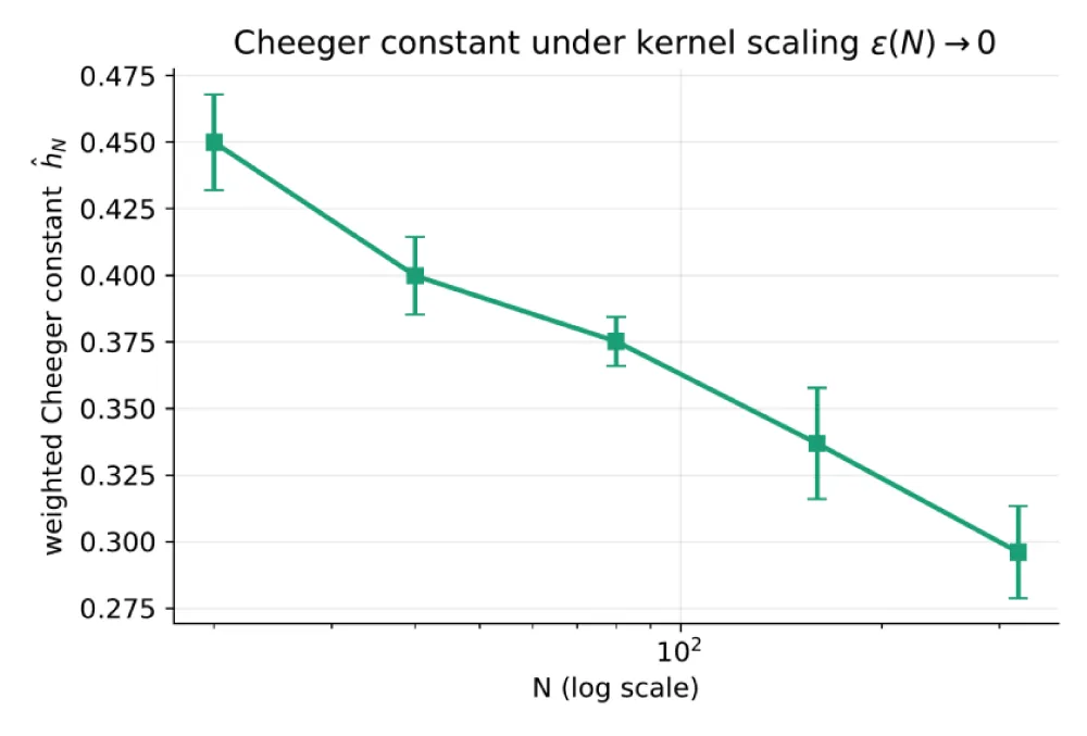The suite now sweeps $N\in \{20,50,100,200\},$ three density regimes (dense/connected, sparse, near-split), and, for tracking, informed fractions $\left|\Gamma \right|/N\in \{0.1,0.2,0.3,0.5\};$  the Cheeger-scaling study of 5 additionally sweeps N up to  under the kernel scaling of 9.

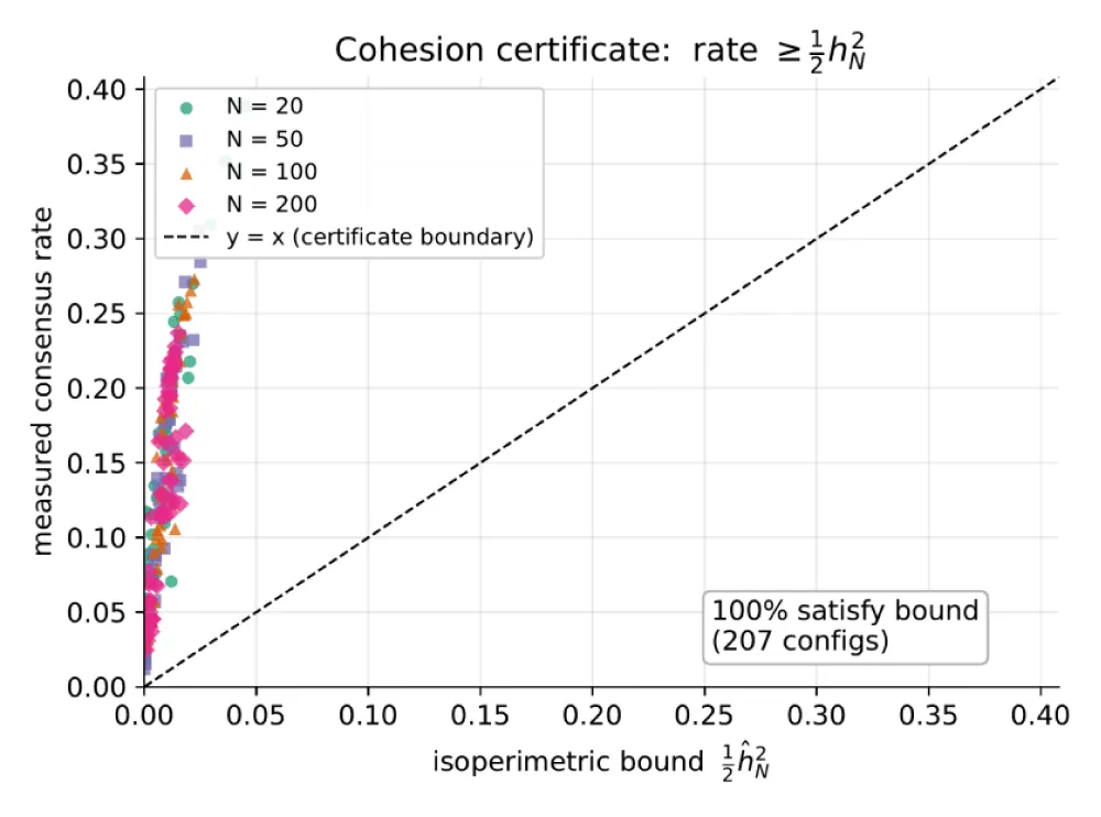
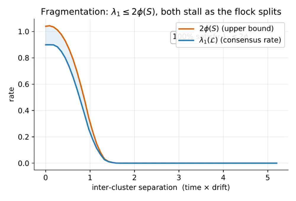
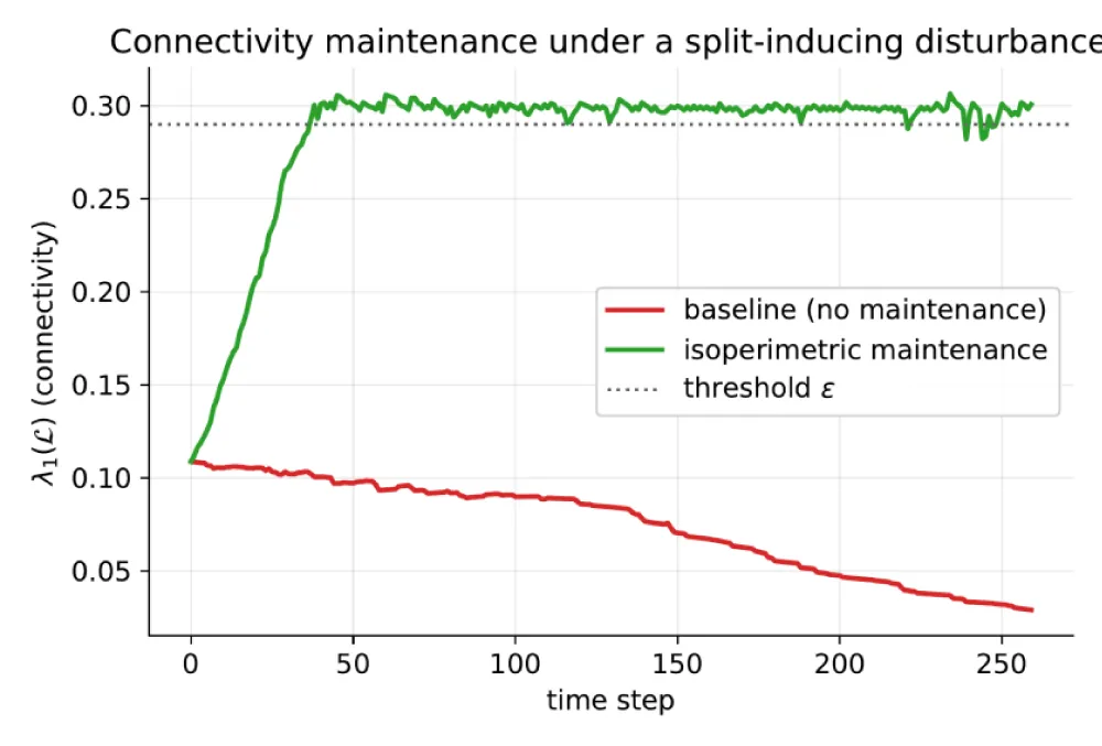
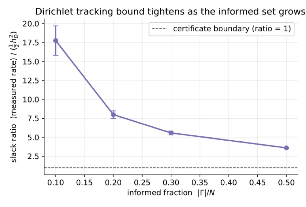
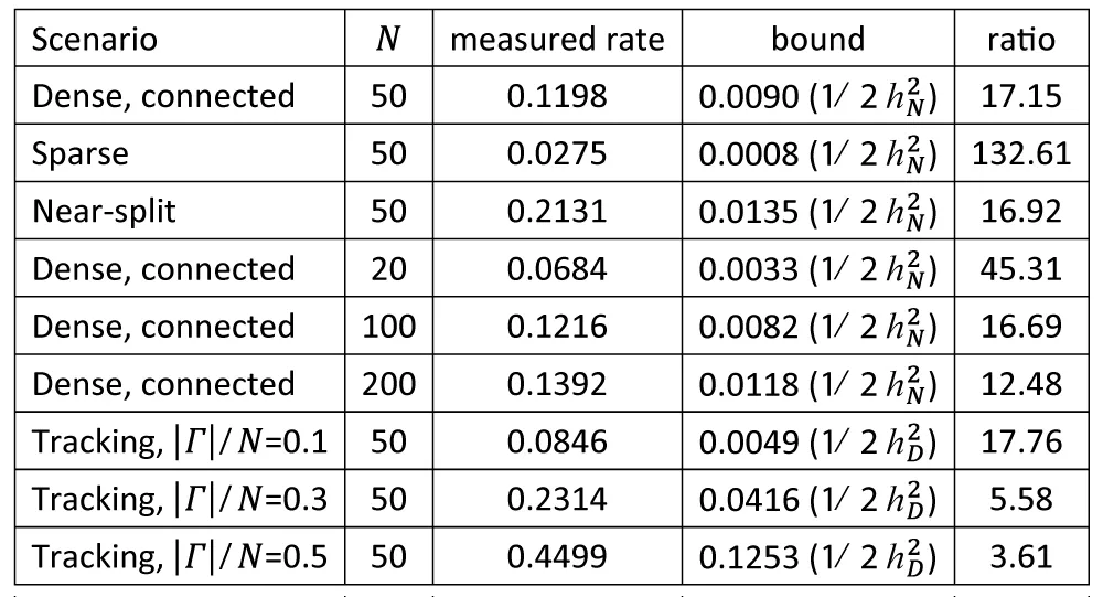
Across  random configurations spanning all four agent counts and three regimes, the cohesion certificate held in every case (1); the fragmentation bound ${\lambda }_1\le 2\varphi \left(S\right)$ held at every step of the forced-split run (2); and the Dirichlet tracking bound held in all  tracking configurations, tightening monotonically as the informed fraction grows (4), consistent with the soft-pinning interpolation of 12 and the tightness analysis of 16. The connectivity-maintenance controller held λ₁ at its threshold where the uncontrolled flock fragmented (3). 1 reports measured rates against the isoperimetric bounds across regimes and agent counts.

Cohesion-rate certificate (6): every measured consensus rate lies above the bound $1/2{\widehat{h}}_N{}^2$ (all points above the diagonal), across $N\in \{20,50,100,200\}$ and three density regimes (207 configurations). The bound is conservative, consistent with the slackness of the lower Cheeger inequality quantified in 16.

Fragmentation early warning (14): λ₁ remains below $2\varphi \left(S\right)$ throughout, and both collapse as the two clusters separate. Here the upper bound is tight, as predicted by 16(1) for a near-balanced cut.

Connectivity maintenance (8): under a split-inducing disturbance the baseline fragments $({\lambda }_1\to 0)$ while the Fiedler-gradient maintenance holds λ₁ at the threshold ∈.

Tracking certificate versus informed fraction. The slack ratio $(measuredrate)/(1/2h_D^2)$ falls from $\sim 18$ at $\left|\Gamma \right|/N=0.1$ toward $\sim 3.6$ at $\left|\Gamma \right|/N=0.5:$ the Dirichlet bound tightens as informed authority grows, matching [prop:soft,prop:tight]. Error bars are standard errors over 12 configurations per fraction.

Weighted Cheeger constant under the kernel scaling of 9, for N up to 320. The finite-N trend is consistent with convergence to a continuum constant (19); establishing the limit rigorously remains open.

Measured convergence rates against the isoperimetric bounds, expanded across regimes and agent counts. All ratios exceed one, confirming the certificates. The cohesion bound is loose ( $\text{ratios}\sim 12-45\times$ for connected graphs, larger near disconnection), while the tracking bound tightens sharply as the informed fraction grows—quantitative support for 16.

The empirical separation between the loose lower (cohesion) bound and the tight upper (fragmentation) bound—now visible across every N and regime—confirms that the early-warning direction is the stronger operational use of the theory, exactly as 16 predicts.

11 Conclusion

We have shown that the weighted isoperimetric inequalities of Chung and Oden [16] furnish geometric certificates for the cohesion, tracking, and fragmentation behavior of second-order flocking dynamics, complementing the spectral viewpoint centered on the algebraic connectivity that dominates the multi-agent literature. The certificates are locally computable, distribute across a swarm with $O\left(\overline{k}\right)$ per-agent communication, and remain valid under a continuously time-varying interaction graph and bounded measurement error; the fragmentation criterion in particular is order-tight and is the operationally strongest instrument the framework provides. Natural extensions include directed and asymmetric sensing (non-self-adjoint Laplacians), time delays and switching topologies, obstacle avoidance as additional Dirichlet boundaries, the fully nonlinear model retaining the separation potential, and stochastic sensing, where the dissipative Laplacian and a noise term are linked by a fluctuation–dissipation relation. The mean-field transfer of 9 remains the central open problem.